Methylize Walkthrough

#Install joblib module for parallelization
import sys
!conda install --yes --prefix {sys.prefix} joblib

Collecting package metadata (current_repodata.json): done
Solving environment: done

# All requested packages already installed.

import methylize
import methylcheck
import numpy as np
import pandas as pd
import matplotlib.pyplot as plt
from statsmodels.stats.multitest import multipletests

Differentially Methylated Position Analysis with Binary Phenotypes

DMPs are probes where methylation levels differ between two groups of samples, while DMRs are genomic regions where DNA methylation levels differ between two groups of samples.

Beta or m-values can be used, but the format needs to be samples as rows and probes as columns.

betas, meta = methylcheck.load_both('../data/asthma') #load in the beta values and metadata
betas = betas.T
print(meta.shape)
meta.head()

INFO:methylcheck.load_processed:Found several meta_data files; attempting to match each with its respective beta_values files in same folders.
WARNING:methylcheck.load_processed:Columns in sample sheet meta data files does not match for these files and cannot be combined:['../data/asthma/sample_sheet_meta_data.pkl', '../data/asthma/GPL13534/GSE157651_GPL13534_meta_data.pkl']
INFO:methylcheck.load_processed:Multiple meta_data found. Only loading the first file.
INFO:methylcheck.load_processed:Loading 40 samples.
Files: 100%|██████████| 1/1 [00:00<00:00,  8.94it/s]
INFO:methylcheck.load_processed:loaded data (485512, 40) from 1 pickled files (0.118s)
INFO:methylcheck.load_processed:Transposed data and reordered meta_data so sample ordering matches.
INFO:methylcheck.load_processed:meta.Sample_IDs match data.index (OK)

(40, 19)

	tissue	disease	smoking_status	passage	Sex	age	description	Sample_ID	Sentrix_ID	Sentrix_Position	Sample_Group	Sample_Name	Sample_Plate	Sample_Type	Sub_Type	Sample_Well	Pool_ID	GSM_ID	Control
20	Airway Fibroblast	Healthy	Ex	4	M	65	fun2norm normalized average beta	9976861129_R03C01	9976861129	R03C01	None	HAF091	None	Unknown	None	None	None	GSM4772065	False
38	Parenchymal Fibroblast	Asthmatic	Non	4	F	19	fun2norm normalized average beta	9976861129_R04C02	9976861129	R04C02	None	7294_P4_LG	None	Unknown	None	None	None	GSM4772083	False
37	Parenchymal Fibroblast	Asthmatic	Non	4	F	14	fun2norm normalized average beta	9976861129_R05C01	9976861129	R05C01	None	7291_lg_p4	None	Unknown	None	None	None	GSM4772082	False
32	Parenchymal Fibroblast	Asthmatic	Current	4	F	15	fun2norm normalized average beta	9976861129_R06C02	9976861129	R06C02	None	7188_lg_p4_R	None	Unknown	None	None	None	GSM4772077	False
23	Airway Fibroblast	Asthmatic	Non	4	F	8	fun2norm normalized average beta	9976861137_R06C01	9976861137	R06C01	None	7016_BR_P4	None	Unknown	None	None	None	GSM4772068	False

Get binary phenotype

The phenotypes can be anything list-like (i.e. a list, numpy array, or Pandas series).

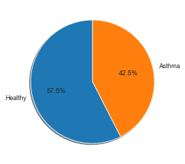
When using Logistic Regression DMP, use phenotype data that is binary (has only 2 classes). In this example, we will take disease state as our phenotype because there are only 2 classes, Asthmatic and Healthy. The DMP step will automatically convert your string phenotype to 0 and 1 if there are not in that format already.

pheno_data = meta.disease
print(pheno_data.shape)
dummies = pd.get_dummies(meta, columns=['disease'])[['disease_Asthmatic', 'disease_Healthy']]
healthy = dummies.disease_Healthy.sum()
asthma = dummies.disease_Asthmatic.sum()
fig1, ax1 = plt.subplots()
ax1.pie((healthy, asthma), labels=['Healthy', 'Asthma'], autopct='%1.1f%%',
        shadow=True, startangle=90)
plt.show()

(40,)

DMP Function

This function searches for individual differentially methylated positions/probes (DMPs) by regressing the methylation beta or M-value for each sample at a given genomic location against the phenotype data for those samples. In this first example, we are using the argument regression_method="logistic" because we are using binary phenotypes.

impute argument:

• Default: ‘delete’ probes if any samples have missing data for that probe.
• True or ‘auto’: if <30 samples, deletes rows; if >=30 samples, uses average.
• False: don’t impute and throw an error if NaNs present ‘average’ - use the average of probe values in this batch ‘delete’ - drop probes if NaNs are present in any sample
• ‘fast’ - use adjacent sample probe value instead of average (much faster but less precise)

Note: if you want to analyze every probe in your betas dataframe, remove the .sample(N). What this does is randomly samples N probes from your dataframe and decreases the time it takes to complete this analysis.

test_results = methylize.diff_meth_pos(betas.sample(20000, axis=1), pheno_data, regression_method="logistic", export=False)
print(test_results.shape)
test_results.head()

WARNING:methylize.diff_meth_pos:Dropped 2902 probes with missing values from all samples

All samples with the phenotype (Asthmatic) were assigned a value of 0 and all samples with the phenotype (Healthy) were assigned a value of 1 for the logistic regression analysis.

(17098, 6)

	Coefficient	StandardError	PValue	95%CI_lower	95%CI_upper	FDR_QValue
cg22048228	-0.320912	0.654584	0.623955	-0.962050	1.603874	0.999978
cg19366543	0.048680	1.217084	0.968095	-2.434121	2.336761	0.999978
cg12408293	-0.070025	1.835602	0.969570	-3.527689	3.667739	0.999978
cg08640790	-0.043054	2.412119	0.985759	-4.684612	4.770720	0.999978
cg02835494	0.027930	1.860959	0.988025	-3.675343	3.619483	0.999978

Differentially Methylated Positions Analysis with Continuous Numeric Phenotypes

Get Continuous Numeric Phenotype

In order to find DMPs against a numeric continuous phenotype, the linear regression method must be used.

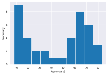
In this example, we are using age as the continuous numeric phenotype.

pheno_data = meta.age.astype(int)
print(pheno_data.shape)
(pheno_data.sort_values()).hist()
plt.xlabel('Age (years)'); plt.ylabel('Frequency')

(40,)

Text(0, 0.5, 'Frequency')

DMP Function

In this second example, we are using the argument regression_method="linear" because we are using continuous numeric phenotypes.

test_results2 = methylize.diff_meth_pos(betas, pheno_data, regression_method="linear", export=False)
print(test_results2.shape)
test_results2.head()

WARNING:methylize.diff_meth_pos:Dropped 71139 probes with missing values from all samples

(414373, 7)

	Coefficient	StandardError	PValue	95%CI_lower	95%CI_upper	Rsquared	FDR_QValue
cg03555227	0.004583	0.000380	1.453304e-14	0.890321	0.890629	0.792946	6.022099e-09
cg16867657	0.008122	0.000718	9.888059e-14	0.877810	0.878454	0.771117	2.048672e-08
cg11169102	-0.004757	0.000460	1.323437e-12	-0.859258	-0.858785	0.737918	1.550767e-07
cg16909962	0.009223	0.000903	1.871221e-12	0.855763	0.856707	0.733140	1.550767e-07
cg23045594	0.005227	0.000511	1.856802e-12	0.856031	0.856566	0.733247	1.550767e-07

To BED

This function converts the stats dataframe from the DMP function into BED format. For more information regarding this function and its arguments, please view the API Reference.

bed = methylize.to_BED(test_results2, manifest_or_array_type='450k', save=False, filename='test_bed.bed')
bed.head()

INFO:methylprep.files.manifests:Reading manifest file: HumanMethylation450k_15017482_v3.csv

	chrom	chromStart	chromEnd	pvalue	name
0	1	69591.0	69641.0	0.060267	cg21870274
1	1	864703.0	864753.0	0.164362	cg08258224
2	1	870161.0	870211.0	0.473560	cg16619049
3	1	877159.0	877209.0	0.267582	cg18147296
4	1	898803.0	898853.0	0.283629	cg13938959

Manhattan Plots

After we run the DMP analysis, we can move on to visualizing the results. One way to do this is a Manhattan plot.

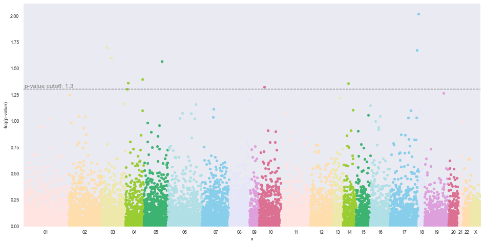
A Manhattan plot has probe position on the x-axis (grouped and colored by chromosome) and -log(p-value) on the y-axis. Because of the scale on the y-axis, the greater the probe is on the y-axis, the more significant that probe is to the phenotype that was used. It is common to have a cutoff on Manhattan plots where we set our α, which commonly is 0.05. Other common α are 0.01 and 0.001. The lower your α is, the more significant probes are that are above that cufoff on the Manhattan plot. The cutoff is for the p-values, meaning the probe is statistically significant if the p-value < α.

Because there are a high number of probes, a p-value correction is needed to prevent false positives. The Manhattan plot function automatically applies a Bonferroni correction to the cutoff to lower the α (increase the dotted cutoff line on the plot) to a more conservative value. The post-test correction is controlled by the adjust argument, where "bonferroni" is the default, and other options are "fdr" for an FDR correction, and None for no post-test correction to keep the cutoff the same as is entered in the cutoff argument.

Manhattan Plot for Binary Phenotypes

methylize.manhattan_plot(test_results, cutoff=0.05, palette='default', save=False, array_type='450k', adjust=None)

INFO:methylprep.files.manifests:Reading manifest file: HumanMethylation450k_15017482_v3.csv

Total probes to plot: 17098
01 1692 | 02 1214 | 03 903 | 04 691 | 05 900 | 06 1275 | 07 1029 | 08 755 | 09 357 | 10 825 | 11 1086 | 12 830 | 13 396 | 14 477 | 15 538 | 16 747 | 17 1058 | 18 221 | 19 904 | 20 392 | 21 144 | 22 304 | X 360

Find Significant Probes

To see which probes are significant (above the cutoff line in the Manhattan plot), filter the results dataframe by the p-value. Because we set post_test=None in the arguments, this means the p-value cutoff that was set is correct, and there was no correction to this value. The next DMR example will have a p-value correction.

interesting_probes = test_results[test_results['PValue'] <= 0.05]
interesting_probes

	Coefficient	StandardError	PValue	95%CI_lower	95%CI_upper	FDR_QValue	minuslog10pvalue	chromosome	MAPINFO
cg11703729	-1.403577	0.708667	0.047638	0.014614	2.792539	0.999978	1.322049	10	CHR-13809615.0
cg01096199	-1.518270	0.754115	0.044082	0.040232	2.996308	0.999978	1.355743	14	CHR-89724701.0
cg14543255	-1.834690	0.796496	0.021254	0.273586	3.395794	0.999978	1.672569	17	CHR-9002458.0
cg26494916	1.621125	0.733396	0.027075	-3.058554	-0.183696	0.999978	1.567434	05	CHR-149453321.0
cg27196131	1.991505	0.985877	0.043380	-3.923787	-0.059222	0.999978	1.362712	04	CHR-187176529.0
cg07351758	1.814658	0.810237	0.025113	-3.402694	-0.226623	0.999978	1.600105	03	CHR-59766624.0
cg23103043	1.830804	0.707215	0.009632	-3.216920	-0.444688	0.999978	2.016264	17	CHR-71650582.0
cg25314266	1.448918	0.706773	0.040360	-2.834168	-0.063668	0.999978	1.394050	04	CHR-76188042.0
cg07538039	1.761092	0.897471	0.049730	-3.520103	-0.002081	0.999978	1.303385	04	CHR-15374511.0
cg21664636	-1.624543	0.698487	0.020029	0.255533	2.993553	0.999978	1.698338	03	CHR-70383513.0

Manhattan Plot for Continuous Numeric Phenotypes

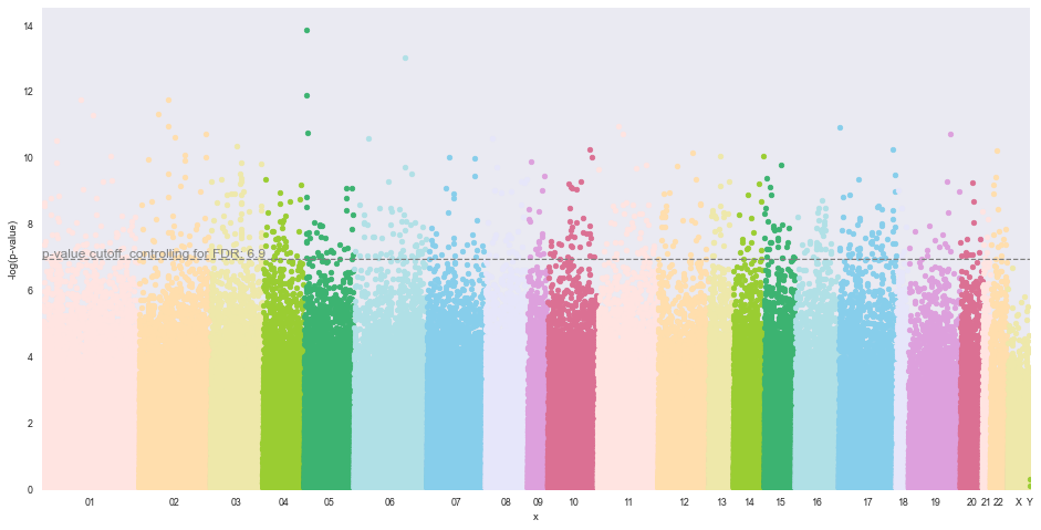
For this example, there will be a Benferoni post-test correction. The adjusted p-value cutoff is displayed on the horizontal cutoff line as well as printed above the plot. Please note that this value is the -log(p-value) of the p-value cutoff.

methylize.manhattan_plot(test_results2, cutoff=0.05, palette='default', save=False, array_type='450k', verbose=True)

INFO:methylprep.files.manifests:Reading manifest file: HumanMethylation450k_15017482_v3.csv

Total probes to plot: 414373
01 40528 | 02 30059 | 03 21877 | 04 17328 | 05 20851 | 06 30620 | 07 24564 | 08 17814 | 09 8501 | 10 20863 | 11 25272 | 12 21229 | 13 10370 | 14 12956 | 15 12921 | 16 18404 | 17 24069 | 18 5215 | 19 21756 | 20 9259 | 21 3329 | 22 7167 | X 9419 | Y 2
p-value cutoff adjusted: 1.3010299956639813 ==[ Bonferoni ]==> 6.9184214452654755

Find Significant Probes

For this Manhattan plot, there has been a p-value cuttoff correction, meaning that the cutoff line is at a more conservative value (lower p-value, higher cutoff line) to account for false positives. Because of this correction, when filtering the results dataframe to find significant probes, you need to filter by the Bonferoni (or FDR) adjust p-value to find the probes above the cutoff line on the Manhattan plot.

adjusted = multipletests(test_results2.PValue, alpha=0.05)
pvalue_cutoff_y = -np.log10(adjusted[3])
interesting_probes2 = test_results2[test_results2['minuslog10pvalue'] >= pvalue_cutoff_y] #bonferoni correction for cutoff
interesting_probes2

	Coefficient	StandardError	PValue	95%CI_lower	95%CI_upper	Rsquared	FDR_QValue	minuslog10pvalue	chromosome	MAPINFO
cg03555227	0.004583	0.000380	1.453304e-14	0.890321	0.890629	0.792946	6.022099e-09	13.837644	05	CHR-170862066.0
cg16867657	0.008122	0.000718	9.888059e-14	0.877810	0.878454	0.771117	2.048672e-08	13.004889	06	CHR-11044644.0
cg11169102	-0.004757	0.000460	1.323437e-12	-0.859258	-0.858785	0.737918	1.550767e-07	11.878297	05	CHR-170858836.0
cg16909962	0.009223	0.000903	1.871221e-12	0.855763	0.856707	0.733140	1.550767e-07	11.727875	01	CHR-229270964.0
cg23045594	0.005227	0.000511	1.856802e-12	0.856031	0.856566	0.733247	1.550767e-07	11.731235	02	CHR-71276753.0
...	...	...	...	...	...	...	...	...	...	...
cg04091914	-0.003923	0.000604	1.185223e-07	-0.726027	-0.724906	0.526302	6.947979e-05	6.926200	02	CHR-227686822.0
cg25874108	-0.002309	0.000355	1.190858e-07	-0.725717	-0.725057	0.526186	6.947979e-05	6.924140	17	CHR-74896813.0
cg01235463	-0.002696	0.000415	1.188893e-07	-0.725800	-0.725029	0.526227	6.947979e-05	6.924857	10	CHR-91154018.0
cg11126313	-0.001694	0.000261	1.199705e-07	-0.725505	-0.725020	0.526006	6.972307e-05	6.920925	03	CHR-46242771.0
cg04161137	-0.003023	0.000465	1.199026e-07	-0.725704	-0.724839	0.526020	6.972307e-05	6.921172	01	CHR-22647687.0

713 rows × 10 columns

Volcano Plot

Logistic Regression Volcano Plots are under construction

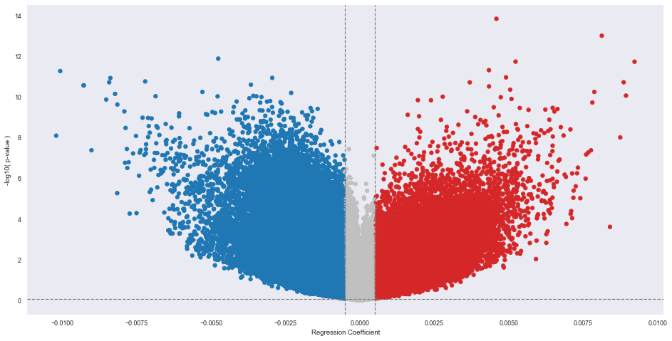
Below shows how to create a Volcano plot using the linear regression DMR analysis.

Positive correlation (hypermethylated) in red. Negative correclation (hypomethylated) in blue

A higher |Regression (beta) coefficient| means that that specific probe is more significant in predicting if the probe is methylated (positive) vs not methylated (negative). The non-gray probes are the probes that are statistically significant, and have a higher absolute value of the regression coefficient as the cutoff. The red probes further to the right on the plot are hypermethylated with increase in age, and the opposite is true for the blue probes.

Useful Arguments:

• alpha: Default: 0.05 alpha level The significance level that will be used to highlight the most significant adjusted p-values (FDR Q-values) on the plot. This is the horizontal cutoff line you see on the plot.
• cutoff: Default: No cutoff format: a list or tuple with two numbers for (min, max) If specified in kwargs, will exclude values within this range of regression coefficients from being “significant” and put dotted vertical lines on chart. These are the vertical cutoff lines you see on the plot. These cutoffs are dependent on the study and up to the researcher in choosing which cutoff is the most desirable.

methylize.volcano_plot(test_results2, fontsize=16, cutoff=(-0.0005,0.0005), alpha=0.05, save=False)

Excluded 269865 probes outside of the specified beta coefficient range: (-0.0005, 0.0005)

Find Significant Probes

interesting_probes3 = test_results2[(test_results2['FDR_QValue'] <= 0.05) & (np.abs(test_results2['Coefficient']) > 0.0005)]
interesting_probes3

	Coefficient	StandardError	PValue	95%CI_lower	95%CI_upper	Rsquared	FDR_QValue	minuslog10pvalue	chromosome	MAPINFO
cg03555227	0.004583	0.000380	1.453304e-14	0.890321	0.890629	0.792946	6.022099e-09	13.837644	05	CHR-170862066.0
cg16867657	0.008122	0.000718	9.888059e-14	0.877810	0.878454	0.771117	2.048672e-08	13.004889	06	CHR-11044644.0
cg11169102	-0.004757	0.000460	1.323437e-12	-0.859258	-0.858785	0.737918	1.550767e-07	11.878297	05	CHR-170858836.0
cg16909962	0.009223	0.000903	1.871221e-12	0.855763	0.856707	0.733140	1.550767e-07	11.727875	01	CHR-229270964.0
cg23045594	0.005227	0.000511	1.856802e-12	0.856031	0.856566	0.733247	1.550767e-07	11.731235	02	CHR-71276753.0
...	...	...	...	...	...	...	...	...	...	...
cg18227216	-0.000972	0.000331	5.680062e-03	-0.430024	-0.428965	0.184466	4.997593e-02	2.245647	17	CHR-10225251.0
cg16297435	0.001548	0.000528	5.681080e-03	0.428642	0.430330	0.184459	4.997954e-02	2.245569	06	CHR-43060558.0
cg05515570	-0.000716	0.000244	5.681038e-03	-0.429877	-0.429096	0.184459	4.997954e-02	2.245572	10	CHR-28125056.0
cg13346820	-0.001955	0.000667	5.680922e-03	-0.430553	-0.428421	0.184460	4.997954e-02	2.245581	05	CHR-865203.0
cg12773197	-0.001329	0.000453	5.681300e-03	-0.430209	-0.428760	0.184457	4.998041e-02	2.245552	13	CHR-111586326.0

43781 rows × 10 columns

Differentiated Methylized Regions (DMR) Analysis

DMRs are genomic regions where DNA methylation levels differ between two groups of samples, while DMPs are probes where methylation levels differ between two groups of samples. DMR looks at clusters or adjacent probes, and if the whole cluster shows the same direction of effect between groups, then it is more significant (likely to be meaningful).

We have already ran methylize.diff_meth_pos with the continuous numeric phenotypes, and the statistics for that fuction is stored in the dataframe test_restuls2. This is what we will use in the DMR function below.

This following step should create these files: * dmr.acf.txt

• dmr.args.txt
• dmr.fdr.bed.gz
• dmr.manhattan.png
• dmr.regions-p.bed.gz
• dmr.slk.bed.gz
• dmr_regions.csv
• dmr_regions_genes.csv
• dmr_stats.csv
• stats.bed

This could run for a while. This function compares all of the probes and clusters CpG probes that show a difference together if they are close to each other in the genomic sequence.

There are many adjustible parameters for the following function, and you can refer to the API Reference for more information.

files_created = methylize.diff_meth_regions(test_results2, '450k', prefix='../data/asthma/dmr/')

INFO:methylprep.files.manifests:Reading manifest file: HumanMethylation450k_15017482_v3.csv
INFO:methylprep.files.manifests:Reading manifest file: HumanMethylation450k_15017482_v3.csv
/Users/jaredmeyers/opt/anaconda3/lib/python3.8/site-packages/methylize/diff_meth_regions.py:150: DtypeWarning: Columns (0) have mixed types.Specify dtype option on import or set low_memory=False.
  results = _pipeline(kw['col_num'], kw['step'], kw['dist'],
Calculating ACF out to: 453
with 17 lags: [1, 31, 61, 91, 121, 151, 181, 211, 241, 271, 301, 331, 361, 391, 421, 451, 481]
18581032 bases used as coverage for sidak correction
INFO:methylize.diff_meth_regions:wrote: ../data/asthma/dmr/.regions-p.bed.gz, (regions with corrected-p < 0.05: 29)
/var/folders/3k/vrkjxj8s7l1gq4x6n7ymqncw0000gn/T/ipykernel_10952/1491901786.py:1: DtypeWarning: Columns (0) have mixed types.Specify dtype option on import or set low_memory=False.
  files_created = methylize.diff_meth_regions(test_results2, '450k', prefix='../data/asthma/dmr/')
INFO:methylize.genome_browser:Loaded 4802 CpG regions from ../data/asthma/dmr/_regions.csv.
INFO:methylize.genome_browser:Using cached `refGene`: /Users/jaredmeyers/opt/anaconda3/lib/python3.8/site-packages/methylize/data/refGene.pkl with (135634) genes
Mapping genes: 100%|██████████| 135634/135634 [00:30<00:00, 4381.01it/s]
INFO:methylize.genome_browser:Wrote ../data/asthma/dmr/_regions_genes.csv

Many of the files created by this function can be useful when using other tools. The file with the main summary of what was just done is found in dmr_regions_genes.csv.

regions_genes = pd.read_csv('../data/asthma/dmr_regions_genes.csv')
regions_genes.head()

	Unnamed: 0	chrom	chromStart	chromEnd	min_p	n_probes	z_p	z_sidak_p	name	genes	distances	descriptions
0	0	1	22289407	22289457	0.03571	1	0.000094	0.7979	cg02053477	NaN	NaN	NaN
1	1	1	34757646	34757696	0.03110	1	0.000054	0.6018	cg13170235	SNRPC	142	Homo sapiens small nuclear ribonucleoprotein p...
2	2	1	34761106	34761156	0.03401	1	0.000081	0.7500	cg15750705	NaN	NaN	NaN
3	3	1	202858152	202858202	0.03110	1	0.000038	0.4790	cg15569630	NaN	NaN	NaN
4	4	10	22334619	22334669	0.03110	1	0.000038	0.4790	cg13327545	NaN	NaN	NaN

This shows clusters of CpG probes that were significantly different and annotes these clusters with mne or more nearby genes using the UCSV Genome Browswer database.

Distances are the number of base-pairs that separate the start of the CpG probe and the start of the coding sequence of the gene.

Only the rows with signicicant p-values will have an annotation.

Adopted from the combined-pvalues package by Brend Pedersen et al, 2013: Comb-p: software for combining, analyzing, grouping and correcting spatially correlated P-values doi: 10.1093/bioinformatics/bts545

More information on DMR on this page

Fetching Genes

This function annotates the DMR region output file using the UCSC Genome Browser database as a reference to what genes are nearby. For more information on this function and the specific argument, please refer to the API Reference

This function can now accept either the filepath or the DMR dataframe output.

reg = pd.read_csv('../data/asthma/dmr_regions.csv')
genes = methylize.fetch_genes('../data/asthma/dmr_regions.csv')
genes.head(12)

INFO:methylize.genome_browser:Loaded 60 CpG regions from ../data/asthma/dmr_regions.csv.
INFO:methylize.genome_browser:Using cached `refGene`: /Users/jaredmeyers/opt/anaconda3/lib/python3.8/site-packages/methylize/data/refGene.pkl with (135634) genes
Mapping genes: 100%|██████████| 135634/135634 [00:28<00:00, 4768.33it/s]
INFO:methylize.genome_browser:Wrote ../data/asthma/dmr_regions_genes.csv

	chrom	chromStart	chromEnd	min_p	n_probes	z_p	z_sidak_p	name	genes	distances	descriptions
0	1	22289407	22289457	0.03571	1	0.000094	0.7979	cg02053477
1	1	34757646	34757696	0.03110	1	0.000054	0.6018	cg13170235	SNRPC	142	Homo sapiens small nuclear ribonucleoprotein p...
2	1	34761106	34761156	0.03401	1	0.000081	0.7500	cg15750705
3	1	202858152	202858202	0.03110	1	0.000038	0.4790	cg15569630
4	10	22334619	22334669	0.03110	1	0.000038	0.4790	cg13327545
5	11	2170376	2170426	0.03110	1	0.000038	0.4790	cg11911653	VARS2	-165,-135	Homo sapiens valyl-tRNA synthetase 2, mitochon...
6	11	2170376	2170426	0.03110	1	0.000038	0.4790	cg14714364	VARS2	-165,-135	Homo sapiens valyl-tRNA synthetase 2, mitochon...
7	11	2346840	2346890	0.04207	1	0.000138	0.9041	cg05532869
8	11	61755269	61755319	0.04150	1	0.000133	0.8968	cg11179625	MYRF	-108	Homo sapiens myelin regulatory factor (MYRF), ...
9	11	69403865	69403915	0.03110	1	0.000068	0.6847	cg05582286	TACR2	-37	Homo sapiens tachykinin receptor 2 (TACR2), mR...
10	11	114063572	114063622	0.03110	1	0.000054	0.6018	cg10096321
11	11	117861576	117861626	0.03110	1	0.000038	0.4790	cg14848289